Most often, you will want to create an Indicators object from a CCF file:

import iCCF

i = iCCF.from_file('r.ESPRE.YYYY-MM-DDTHH:MM:SS.SSS_CCF_A.fits')
# CCFindicators(CCF from r.ESPRE.YYYY-MM-DDTHH:MM:SS.SSS_CCF_A.fits)

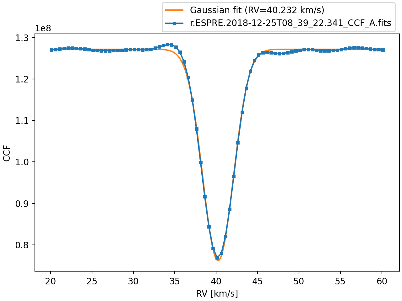
It’s useful to visualize the CCF as well:

i.plot()

Then, the i object stores several CCF indicators as attributes.
The radial velocity and uncertainty are stored in the RV and RVerror attributes

i.RV        # np.float32(40.23212)
i.RVerror   # np.float32(0.0002788162)

In this example, both the radial velocity and the uncertainty are 32-bit floats. This is because the underlying CCF data was stored as 32-bit floats as well. iCCF takes great care to preserve the numerical precision in all calculations.

These values were calculated by fitting a Gaussian function to the CCF, in the same way as done by the ESPRESSO pipeline. We also have access to the original pipeline RV value that is stored in the header of the CCF file:

i.pipeline_RV  # 40.2321199262624

The pipeline value is stored in the header with full 64-bit precision!

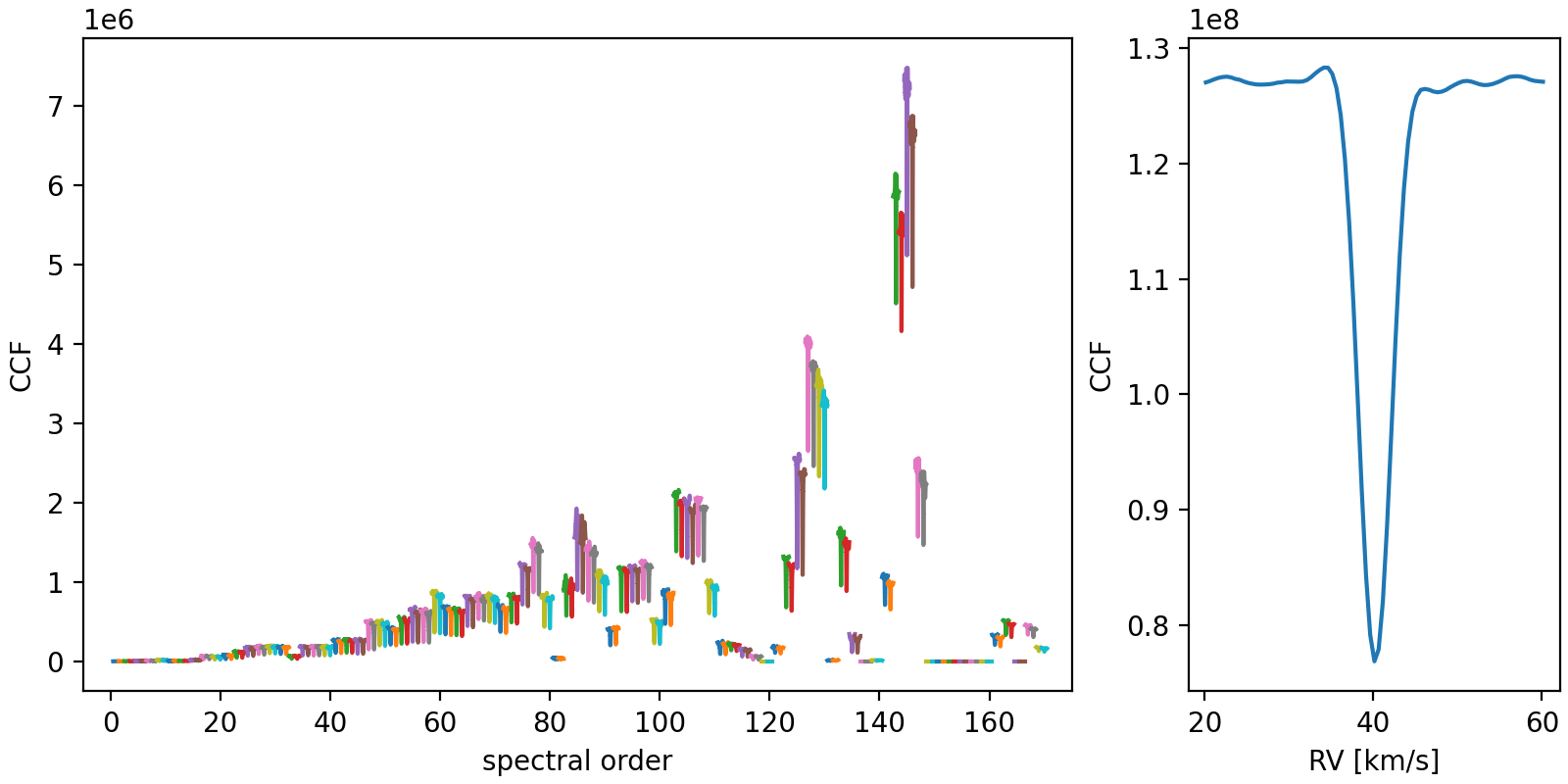
Order-by-order RVs and CCFs

The i object also stores the order-by-order CCFs, which allows to calculate the individual RVs for each order. These can be conveniently accessed via the i.individual_RV attribute and plotted with:

i.plot_individual_RV()

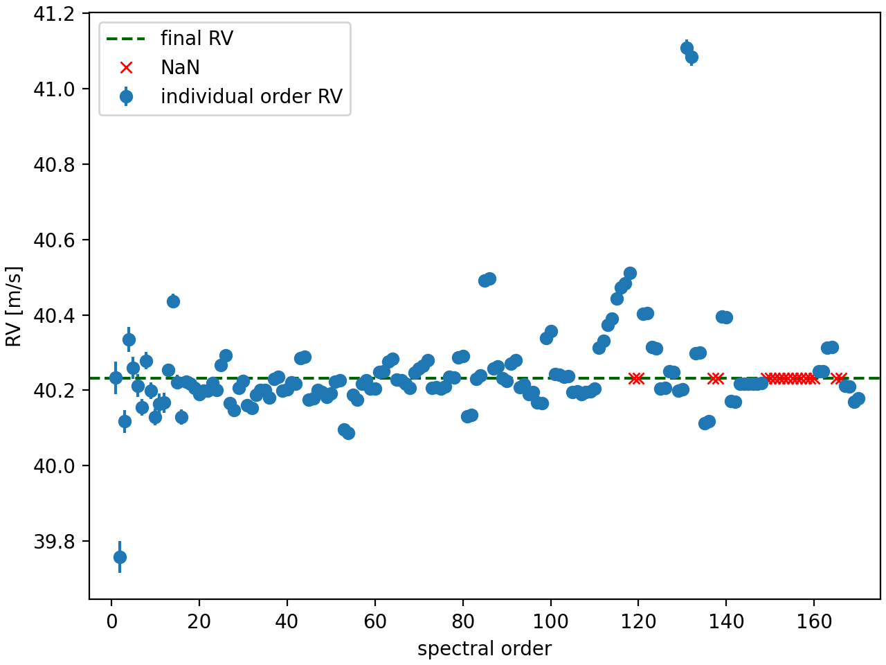
Some of the individual RVs are NaN because that order’s CCF is equal to zero.

In fact, the order-by-order CCFs can also be visualised easily:

i.plot_individual_CCFs()